Next: Simulation results
Up: Estimating the inverse nonlinear
Previous: MLP model
In order to train the MLP weights and biases a cost function is
designed that allows training blindly on the available nonlinear
cluster data. The cost should be minimal when these data are
mapped onto linear clusters by the entire set of MLPs, therefore
ideally there should be a linear relationship between all
components  and
and  within the same cluster
  :
:
 |
(5) |
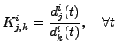
where  is the slope made up by the components and
of cluster . Hence, a cost function to train the weights of
MLP can be derived as
is the slope made up by the components and
of cluster . Hence, a cost function to train the weights of
MLP can be derived as
![$\displaystyle J_j = \sum_{i=1}^n \sum_{k=1}^m \sum_t \left[ d_j^i(t) - K_{j,k}^i d_k^i(t) \right]^2$](img70.png) |
(6) |
Notice that the elements of  must also be estimated and
updated in each iteration, for instance by using the
histogram-based estimator described in [8]. Fig.
1 shows the training diagram
corresponding to the case
must also be estimated and
updated in each iteration, for instance by using the
histogram-based estimator described in [8]. Fig.
1 shows the training diagram
corresponding to the case  .
.
The MLPs are initialized to get a linear input-output
transformation:
 . This
initialization is relatively ``near'' the optimal solution and
prevents the weights from converging to a trivial (all zeroes)
solution. The parameters of the
. This
initialization is relatively ``near'' the optimal solution and
prevents the weights from converging to a trivial (all zeroes)
solution. The parameters of the  MLPs are adapted in each
iteration using a batch gradient descent approach to minimize
(6). And, as suggested in
[13], we also assume that they pass
through the origin, i.e.,
MLPs are adapted in each
iteration using a batch gradient descent approach to minimize
(6). And, as suggested in
[13], we also assume that they pass
through the origin, i.e.,
 ; therefore the bias of the
output layer
; therefore the bias of the
output layer  is fixed as
 . After this training the mixing
matrix can be estimated in a straightforward way relying on the
estimated .
. After this training the mixing
matrix can be estimated in a straightforward way relying on the
estimated .
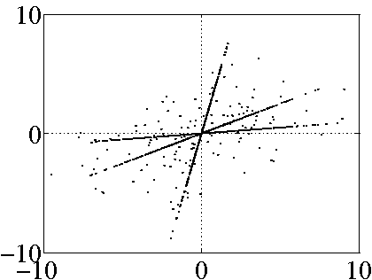
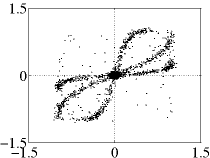
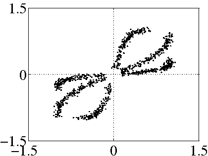
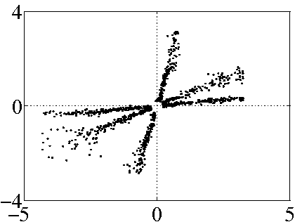
Figure 2:
Example of underdetermined BSS mixtures: scatter plots of
three linear mixtures in (a) and three PNL mixtures with additive
noise in (b), with  and
and  dB SNR. The preprocessing of
Section III removes some samples of (b) to
obtain (c), which is then used for spectral clustering. (d) shows
the output of the MLPs after training with the clustered data.
dB SNR. The preprocessing of
Section III removes some samples of (b) to
obtain (c), which is then used for spectral clustering. (d) shows
the output of the MLPs after training with the clustered data.
|
|
Next: Simulation results
Up: Estimating the inverse nonlinear
Previous: MLP model
Steven Van Vaerenbergh
Last modified: 2006-04-05