


Next: Cost function and parameter
Up: Estimating the inverse nonlinear
Previous: Estimating the inverse nonlinear
To represent each inverse nonlinear function  (
(
 ) we use a single input, single output multilayer
perceptron with one hidden layer of
) we use a single input, single output multilayer
perceptron with one hidden layer of  neurons. Once the samples
are clustered into
neurons. Once the samples
are clustered into  sets by the spectral clustering algorithm,
the elements of each set are used as input patterns for the
sets by the spectral clustering algorithm,
the elements of each set are used as input patterns for the  MLPs. In particular, for the
  -th cluster we have patterns
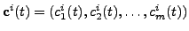 , where
  is a
discrete time unit. The
is a
discrete time unit. The  -th component of each pattern is fed
into the -th MLP, whose output is given by
-th component of each pattern is fed
into the -th MLP, whose output is given by
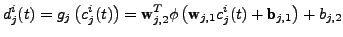 |
(4) |
where
 are weight vectors,
 and
and
 are biases and
  is a
neuron activation function. For all the neurons in the hidden
layers we chose to use the hyperbolic tangent activation function.
is a
neuron activation function. For all the neurons in the hidden
layers we chose to use the hyperbolic tangent activation function.
Figure 1:
The block diagram used for the MLP parameter training for
 . The blocks labelled
  and
and  represent the two
MLPs. The slope estimator is used to estimate the slope
represent the two
MLPs. The slope estimator is used to estimate the slope
 of the curve formed by
 . To train
the upper MLP, we use as desired signal
. To train
the upper MLP, we use as desired signal
 . In
this way the error signal
. In
this way the error signal
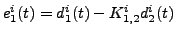 measures the deviation from linearity of this curve. The
same procedure is carried out for the lower MLP.
measures the deviation from linearity of this curve. The
same procedure is carried out for the lower MLP.
|
|
Next: Cost function and parameter
Up: Estimating the inverse nonlinear
Previous: Estimating the inverse nonlinear
Steven Van Vaerenbergh
Last modified: 2006-04-05
