


Next: Dividing the samples into
Up: Problem Statement
Previous: Linear mixture model
In a realistic scenario the  sensors that measure the mixtures
show some kind of nonlinearity, which suggests the extension of
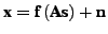
(2) to a post-nonlinear mixture model
sensors that measure the mixtures
show some kind of nonlinearity, which suggests the extension of
(2) to a post-nonlinear mixture model
 |
(3) |
where
![$ \textbf{f}(\cdot) = [f_1(\cdot), f_2(\cdot), \dots,
f_m(\cdot) ]^T$](img32.png) is a componentwise nonlinear function and
is a componentwise nonlinear function and
 is the measurement random
vector. For the underdetermined case (
is the measurement random
vector. For the underdetermined case ( ) the methods from
linear BSS are not able to estimate the sources properly. A
scatter plot example of PNL mixtures is shown in Fig.
2(b).
) the methods from
linear BSS are not able to estimate the sources properly. A
scatter plot example of PNL mixtures is shown in Fig.
2(b).
The proposed algorithm aims at estimating the inverse
nonlinearities
 , under the condition
that they are invertible and linear for small input values. This
leads directly to an estimate of the linear mixtures
, under the condition
that they are invertible and linear for small input values. This
leads directly to an estimate of the linear mixtures
 , which can be used to recover
the original sources
, which can be used to recover
the original sources
 relying on known methods for
underdetermined linear BSS.
relying on known methods for
underdetermined linear BSS.
Steven Van Vaerenbergh
Last modified: 2006-04-05