System Identification

An important characteristic of the Wiener system is that its linear filter is usually time-varying. Whereas the identification method of Section III will reliably identify the different blocks of a static system as a batch method, an online approach is required to track the time-variations of a Wiener system.

An online prediction setup assumes we are given a stream of input-output pairs $\{(\textbf{x}_1[n],x_2[n]), (\textbf{x}_1[n-1],x_2[n-1]), \dots\}$, in which every $\textbf{x}_1[n] = (x_1[n],x_1[n-1],\dots,x_1[n-L+1])^T$ is a vector representing a memory of the length of the linear filter $H(z)$. A key feature of online algorithms is that the number of computations must not increase as the number of samples increases. Since the size of a kernel matrix depends on the number of samples used to calculate it, we chose to take into account only a ``sliding-window'' containing the last $N$ input-output pairs of this stream. For window $n$, the observation matrix $\textbf{X}_1^{(n)} = (\textbf{x}_1[n], \textbf{x}_1[n-1], \dots, \textbf{x}_1[n-N+1])^T$ and the observation vector $\textbf{x}_2^{(n)} = (x_2[n], x_2[n-1], \dots, x_2[n-N+1])^T$ are formed and the corresponding kernel matrix $\textbf{K}^{(n)} = \textbf{\~x}_2^{(n)}(\textbf{\~x}_2^{(n)})^T$ and regularized kernel matrix $\textbf{K}_{reg}^{(n)} = \textbf{K}^{(n)}+ c\textbf{I}$ can be calculated.

To solve (9), in each iteration the $N\times N$ inverse matrix $(\textbf{K}_{reg}^{(n)})^{-1}$ must be calculated. This is costly both computationally and memory-wise (requiring $O(N^3)$ operations). Therefore in [14] an update algorithm was developed that can compute $(\textbf{K}_{reg}^{(n)})^{-1}$ solely from knowledge of the data of the current observation vector $\textbf{x}_2^{(n)}$ and the previous $(\textbf{K}_{reg}^{(n-1)})^{-1}$.

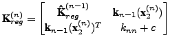
Given the kernel matrix $\textbf{K}_{reg}^{(n-1)}$, the new kernel matrix $\textbf{K}_{reg}^{(n)}$ can be constructed by removing the first row and column of $\textbf{K}_{reg}^{(n-1)}$, referred to as $\textbf{\^K}_{reg}^{(n-1)}$, and adding kernels of the new data as the last row and column:

$$\textbf{K}_{reg}^{(n)} = \begin{bmatrix}\textbf{\^K}_{reg}^{(n-1)... ...f{x}_2^{(n)})\\ \textbf{k}_{n-1}(\textbf{x}_2^{(n)})^T & k_{nn}+c \end{bmatrix}$$ (10)

with $\textbf{k}_{n-1} (\textbf{x}_2^{(n)}) = [\kappa(\textbf{x}_2^{(n-N+1)}, \textbf{x}_2^{(n)}), \dots, \kappa(\textbf{x}_2^{(n-1)}, \textbf{x}_2^{(n)})]^T$ and $k_{nn} = \kappa(\textbf{x}_2^{(n)}, \textbf{x}_2^{(n)})$.

Calculating the inverse kernel matrix $(\textbf{K}_{reg}^{(n)})^{-1}$ is done in two steps, using the two inversion formulas from the appendix at the end of this paper. Note that these formulas do not calculate the inverse matrices explicitly, but rather derive them from known matrices maintaining an overall time and memory complexity of $O(N^2)$ of the algorithm.

First, given $\textbf{K}_{reg}^{(n-1)}$ and $(\textbf{K}_{reg}^{(n-1)})^{-1}$, the inverse of the $N-1\times N-1$ matrix $\textbf{\^K}_{reg}^{(n-1)}$ is calculated according to Eq. (12). Then $(\textbf{K}_{reg}^{(n)})^{-1}$ can be calculated applying the matrix inversion formula from Eq. (11), based on the knowledge of $(\textbf{K}_{reg}^{(n-1)})^{-1}$ and $\textbf{K}_{reg}^{(n)}$.

The complete algorithm to solve (9) in an adaptive manner is summarized in Alg. (1).