Kernel Canonical Correlation Analysis

Although CCA constitutes a good technique to find linear relationships between two or several [17] data sets, it is not able to extract nonlinear relationships. In order to solve this problem, CCA has been extended to nonlinear CCA and kernel-CCA (K-CCA) [11,12,19]. Specifically, kernel CCA exploits the characteristics of kernel methods, consisting in the implicit nonlinear transformation of the data $\textbf{x}_i$ from the input space to a high dimensional feature space $\tilde{{\mathbf x}}_i = \Phi(\textbf{x}_i)$. Then, solving CCA in the feature space we are able to extract nonlinear relationships.

The key property of the kernel methods and reproducing kernel Hilbert spaces (RKHS) is that, since the scalar products in the feature space can be seen as nonlinear (kernel) functions of the data in the input space, the explicit mapping to the feature space can be avoided, and any linear technique can be performed in the feature space by solely replacing the scalar products by the kernel function in the input space. In this way, any positive definite kernel function satisfying Mercer's condition [20]: $\kappa(\textbf{x}_i,\textbf{x}_j) = \langle \Phi(\textbf{x}_i),\Phi(\textbf{x}_j) \rangle$ has an implicit mapping to some higher-dimensional feature space. This simple and elegant idea is known as the ``kernel trick'', and it is commonly applied by using a nonlinear kernel such as the Gaussian kernel

$$\kappa(\textbf{x},\textbf{y}) = \exp \left( -\frac{\Vert\textbf{x}-\textbf{y}\Vert^2}{2\sigma^2} \right),$$

which implies an infinity-dimensional feature space.

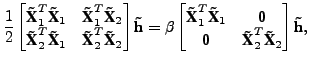
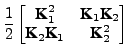
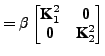
After transforming the data and canonical vectors to feature space, the GEV problem (3) can be written as

$$\frac{1}{2} \begin{bmatrix}\textbf{\~X}_1^T \textbf{\~X}_1 & \tex... ...f{0}\\ \textbf{0} & \textbf{\~X}_2^T \textbf{\~X}_2 \end{bmatrix} \textbf{\~h},$$ (4)

where $\textbf{\~X}_k \in \mathbb{R}^{N\times m_k'}$ represents the transformed data and $\textbf{\~h} = [\textbf{\~h}_1^T \textbf{\~h}_2^T]^T$ contains the transformed canonical vectors of length $m_1'$ and $m_2'$. Taking into account that the canonical vectors $\textbf{\~h}_1$ and $\textbf{\~h}_2$ belong to the subspace defined by the rows of $\textbf{\~X}_1$ and $\textbf{\~X}_2$ respectively we can find two vectors $\alpha$$_k \in \mathbb{R}^{N \times 1}$ such that

$$\textbf{\~h}_k = \textbf{\~X}_k^T \mbox{\boldmath$\alpha$\unboldmath } _k \quad k=1,2,$$

and left-multiplying (4) by

$$\begin{bmatrix}\textbf{\~X}_1 & \textbf{0}\\ \textbf{0} & \textbf{\~X}_2 \end{bmatrix}$$

we obtain

$$\frac{1}{2} \begin{bmatrix}\textbf{K}_1^2 & \textbf{K}_1 \textbf{K}_2\\ \textbf{K}_2 \textbf{K}_1 & \textbf{K}_2^2 \end{bmatrix} \mbox{\boldmath$\alpha$\unboldmath } = \beta \begin{bmatrix}\textbf{K}_1^2 & \textbf{0}\\ \textbf{0} & \textbf{K}_2^2 \end{bmatrix} \mbox{\boldmath$\alpha$\unboldmath } ,$$ (5)

where ${\mathbf K}_k = \textbf{\~X}_k \textbf{\~X}_k^T$ is the kernel matrix with elements

$$\textbf{K}_k(i,j) = \kappa_k({\mathbf x}_k[i],{\mathbf x}_k[j]),$$

in its $i$-th row and $j$-th column, $\kappa_k(\cdot,\cdot)$ is the kernel applied to the $k$-th data set, and ${\mathbf x}_k^T[i]$ denotes the $i$-th row of the $k$-th data matrix. Finally, (5) can be simplified to

$$\frac{1}{2} \begin{bmatrix}\textbf{K}_1 & \textbf{K}_2\\ \textbf{K}_1 & \textbf{K}_2 \end{bmatrix} \mbox{\boldmath$\alpha$\unboldmath } = \beta \begin{bmatrix}\textbf{K}_1 & \textbf{0}\\ \textbf{0} & \textbf{K}_2 \end{bmatrix} \mbox{\boldmath$\alpha$\unboldmath } ,$$ (6)

and the resulting GEV constitutes again two coupled kernel-LS regression problems defined now as

$$J_k(\beta \mbox{\boldmath$\alpha$\unboldmath } _k) = \Vert {\mathbf K}_k \beta \mbox{\boldmath$\alpha$\unboldmath } _k - {\mathbf y}\Vert^2 \quad k=1,2,$$

where ${\mathbf y}_k = {\mathbf K}_k$   $\alpha$$_k$ and ${\mathbf y}= ({\mathbf y}_1+{\mathbf y}_2)/2$ is the desired output.

To summarize, the application of the kernel trick permits the solution of the CCA problem in the feature space without increasing the computational cost and conserving the LS regression framework.