Kernel Methods

The linear LS methods can be extended to nonlinear versions by transforming the data into a feature space. Using the transformed vector $\textbf{\~h} \in \mathbb{R}^{M'\times 1}$ and the transformed data matrix $\textbf{\~X} \in \mathbb{R}^{N\times M'}$, the LS problem (2) can be written in feature space as

$$J' = \min_{\textbf{\~h}} \Vert\textbf{y} - \textbf{\~X} \textbf{\~h} \Vert^2.$$ (3)

The transformed solution $\textbf{\~h}$ can now also be represented in the basis defined by the rows of the (transformed) data matrix $\textbf{\~X}$, namely as

$$\textbf{\~h} = \textbf{\~X}^T \mbox{\boldmath$\alpha$\unboldmath } .$$ (4)

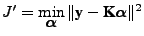
Moreover, introducing the kernel matrix $\textbf{K} = \textbf{\~X} \textbf{\~X}^T$ the LS problem in feature space (3) can be rewritten as

$$J' = \min_{\mbox{\boldmath$\alpha$\unboldmath }} \Vert\textbf{y} - \textbf{K} \mbox{\boldmath$\alpha$\unboldmath } \Vert^2$$ (5)

in which the solution $\alpha$ is an $N\times 1$ vector. The advantage of writing the nonlinear LS problem in the dual notation is that thanks to the ``kernel trick'', we only need to compute $\textbf{K}$, which is done as

$$\textbf{K}(i,j) = \kappa(\textbf{X}_i,\textbf{X}_j),$$ (6)

where $\textbf{X}_i$ and $\textbf{X}_j$ are the $i$-th and $j$-th rows of $\textbf{X}$. As a consequence the computational complexity of operating in this high-dimensional space is not necessarily larger than that of working in the original low-dimensional space.